Example Applications: Fish Passage at Big Noise Creek

Location:  Big Noise Creek is located in the North Coast basin.  The creek is located in Clatsop County, has headwaters in the Clatsop State Forest at an elevation of approximately 1,200 feet above sea level, flows North under Route 30 and joins Rock Creek which eventually enters the Columbia River. 

Description of Project: The Oregon Department of Transportation (ODOT) is currently (2001-2002) using an existing culvert for experimental retrofitting to improve juvenile fish passage.  The culvert allows Big Noise Creek to flow under Route 30.  This creek does not have a streamflow gage. 

Objectives:  For purposes of illustration, determine peak discharge values for the stream to identify the culvert design flow that could be used to size the culvert.  Determine the range of culvert discharges and their seasonal values that juvenile fish may encounter and use for testing fish-passage design flow. For fish passage concerns, it is necessary that the flows move through the culvert at appropriate velocities for juvenile fish (e.g., 2 ft/s) and maintain a low-flow water depth (e.g., 8 in), based on criteria set by the Oregon Department of Fish and Wildlife (ODFW).

Procedure:

Step1: Review the Preliminary Estimations page to determine a rough estimate of streamflow values for this region.

The preliminary estimates for the North Coast Basin will appear as follows:

Note that the percentages do not quite add up to 100% (sum is 99%) due to rounding of decimal values.

Step 2:  Determine the drainage area of Big Noise Creek from topographic maps (USGS topographic maps, Knappa and Cathlamet Quadrangles).

After delineating the boundary of the Big Noise Creek drainage area on topographic maps, a planimeter was used to determine the drainage area (a GIS could also be used for this purpose).  The drainage area for Big Noise Creek is approximately 1.8 square miles.

With this drainage area the annual discharge is expected to be approximately 9 cfs.  The annual flow pattern shows low flows during the summer months and high flows during the winter months.  December, January and February have the highest flows.

Step 3:  Identify a nearby gage.

A review of the table of USGS gages for coastal Oregon shows three existing gages that may be used for this project: Bear Creek, Tucca Creek, and Youngs River.  The table below lists information for these gages and also for the Wilson River gage, which will be used later in the example.  Bear Creek and Tucca creek both have small drainage areas similar to the project stream.  Beak Creek and Youngs River are both located in Clatsop county and flow north similar to the project stream. 

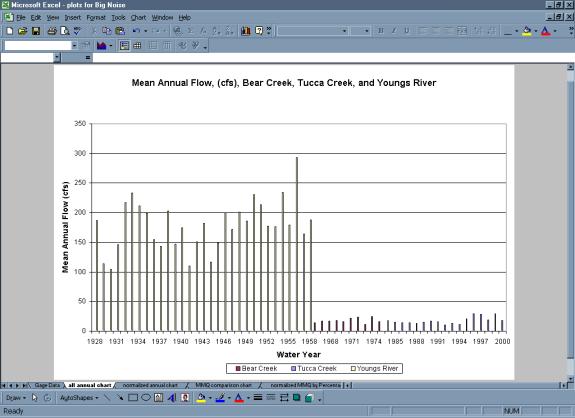
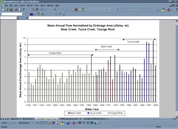
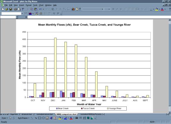
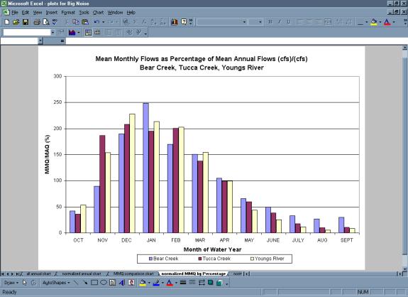
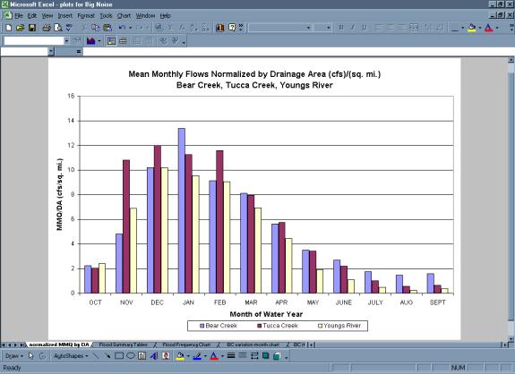
Plots of mean annual flow vs. water year and normalized mean annual flow vs. water year are useful for visualizing the period of record for each gage and the general streamflow pattern for the period of record.  Youngs River has the longer period of record but the drainage area is substantially larger than the project watershed.  Plots of mean monthly flows and normalized mean monthly flows illustrate the yearly streamflow pattern of each stream.  All three streams seem to have large flows in the winter months (Dec, Jan, Feb) and have low flows in the summer months (July, Aug, and Sept).  The plot of mean monthly flows normalized by drainage area shows that for three out of the four winter months (Nov, Dec, Feb) Tucca creek has a larger value of MMQ/DA than Bear Creek.  Bear Creek has the highest MMQ/DA for January and also for the low flow months of July, August and September.  The two creeks, Bear Creek and Tucca Creek, may have slightly different yearly streamflow patterns due to different local precipitation patterns in the regions where they are located.  

At this point, after examining the plots and comparing the stations with site characteristics, the user may be able to select the nearby gage for use of its streamflow data.  An alternative, which is followed here for illustrative purposes, is to conduct the hydrologic evaluations using more than one station.  Although requiring more work, this has the advantage of developing multiple estimates for needed values, which may add confidence that the results are realistic and not anomalous to a particular single selected gage.

Step 4:  Perform a flood frequency analysis to determine peak discharges for various return periods. 

Peak flow analysis was done using data from all three streams.  The results of the flood frequency analysis are listed in the tables and chart that follow.   The flood discharge values calculated for each stream were scaled down to the drainage area of Big Noise Creek using a ratio of drainage areas (DA of Big Noise Creek/DA of nearby gage).

FLOOD FREQUENCY CALCULATIONS USING LOG-PERSON TYPE III ANALYSIS

Instantaneous Peaks

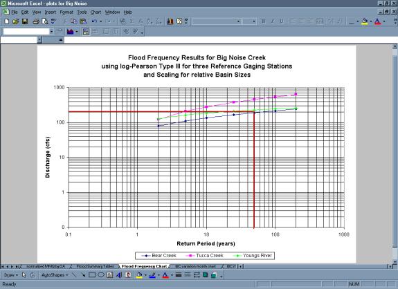
For this example, a 50-year flood will be used as the design discharge.  Both Youngs River and Bear Creek estimate the 50-year flood to be approximately 200 cfs.  The Youngs River estimate is slightly lower than the estimate obtained using data from the gage at Bear Creek.  The drainage area of the Youngs River gaging station is larger than that for the project site.  Smaller watersheds tend to exhibit different flood peak characteristics than larger ones.   Other considerations being equal, usually, time to peak is faster and peak flows for the drainage area are larger.  The Youngs River data may give lower peak flow estimates due to the attenuation of flood peaks in the larger watershed and may not provide a fully accurate representation of the smaller drainage area of the project stream.

Tucca Creek estimates the largest discharge values for each return period.  Tucca creek has a slightly longer period of record compared to Bear Creek but Bear Creek is more geographically similar to the project area.  Tucca Creek has its headwaters in the Coast Range at approximately 1,500 feet above sea level and flows west to join the Nestucca River, which eventually enters the Pacific Ocean.  The precipitation patterns in this region, due to orographic effects along the Coast Range, may be different than at the project site.  Orographic effects cause the rain clouds blowing east from the Pacific Ocean to release their moisture on the western slopes of the Coast Range in manners that are affected by elevation and rate of elevation change.  Because the Coast Range is the first mountain barrier encountered by air masses moving landward from the Pacific, many of the coastal streams have elevated flows compared to other regions of Oregon.  The plot of mean monthly flow normalized by drainage area illustrates that Tucca Creek has larger MMQ/DA than Bear Creek for the winter (wet) months.  Using Tucca Creek data may lead to overestimation of peak flow values.

Thus, although Bear Creek has the smallest period of record, its location and drainage area size may render it the best choice for estimating the streamflow characteristics of Big Noise Creek.  Bear Creek was selected as the appropriate nearby gage to use for hydrologic assessment of Big Noise Creek.  Culvert design is usually based on peak flow analysis.  Oregon Department of Transportation (ODOT) guidelines will usually set the criteria that should be used and the discharge associated with the criteria would be used for the design process.  For example, if the culvert needs to be designed to withstand a 50-year flood, then it must have the capacity to handle a discharge of 212 cfs, based on the foregoing flood frequency analysis.

Step 5:  Perform Monthly Analysis for Big Noise Creek based on Bear Creek Data

In addition to allowing passage for the stream, culverts also need to provide passage for the fish inhabiting the stream.  When performing hydrologic analysis for fish passage evaluations, it is helpful to perform the analysis on a monthly basis.  All analyses for fish passage were done using streamflow data from the gage at Bear Creek and scaling down the values to the drainage area of Big Noise Creek.  Bear Creek streamflow data were scaled using the ratio of the drainage area of Big Noise Creek to the drainage area of Bear Creek (1.8 sq mi. / 3.33 sq mi.).

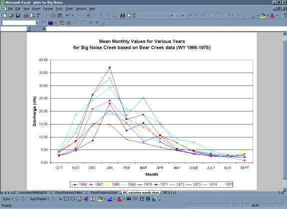
• Discharge vs. Month for various water years
  • Shows the year-to-year variability of the monthly streamflow pattern.  For each month, the past record shows a range of observed flows.

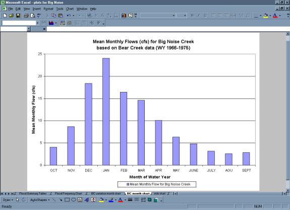
• Discharge vs. Month of the water year
  • Shows the annual streamflow pattern based on averages for each month.  This simplifies the previous graph by eliminating variability through calculation of the mean values, by month.

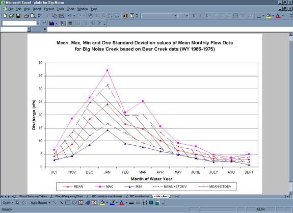
• Discharge vs. Month of the water year with various statistics added (such as the mean, the observed extremes and the standard deviation) to discern the range of flow values to be considered.
  • Allows the user to visualize the range of flows expected to occur and the range for some percent (e.g., 68%) of the time to better know the most common flows.

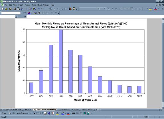
• Mean Monthly Flows as a Percentage of Mean Annual Flow
  • Shows the wet and dry months of the year by the distance above and below the mean annual flow value of 100%.

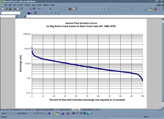
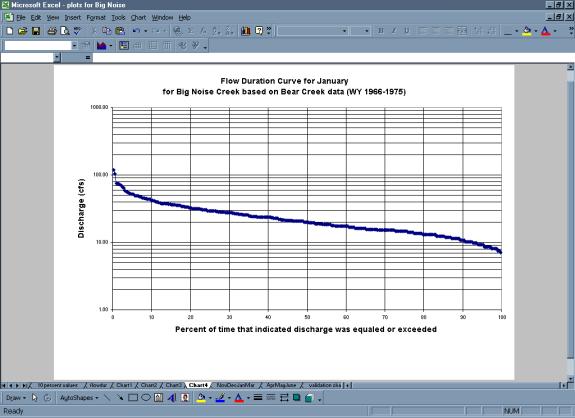
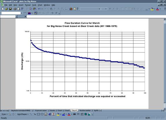
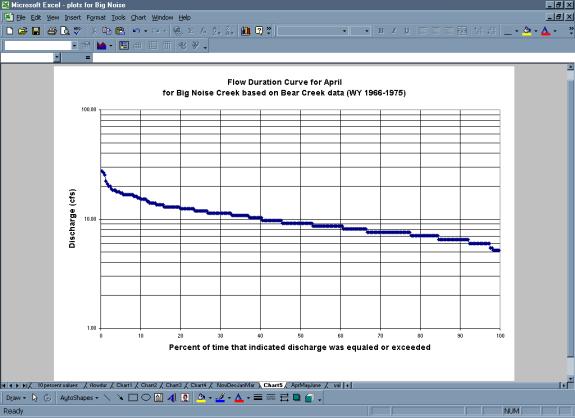
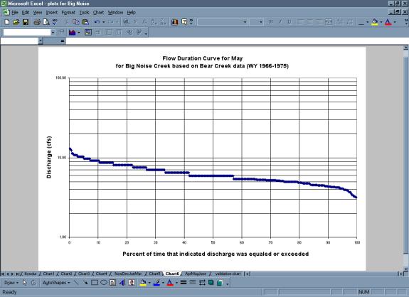
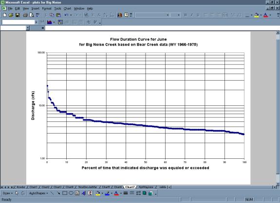
Step 6:  Generate flow duration curves for each month that fish are present and migrating in the creek. 

It is not considered necessary or practical to design culverts to pass fish at all times of year, particularly during brief periods at flood stage.  Fish generally are thought to take refuge when flows are severe and wait out the passage of a flood.  Hence, the hydraulic design of culverts for fish movement includes selection of appropriate design flows from which the corresponding flow characteristics can be derived by hydraulic analysis.  For example, the low flow depth design may be based on the 95% exceedence flow for the migration period of the fish species of concern.  Similarly, the high flow design discharge could be the flow that is not exceeded more than 10% of the time during the months of migration (for current ODFW guidlines, click here).  Flow duration curves should be generated using daily flow values for each month that fish are migrating in the stream to determine the corresponding 95% and 10% exceedence flows.  Fish passage criteria, set by fisheries agencies, indicated that all of these flows must be able to pass through the conventional culvert at a specified maximum velocity (e.g. 2 ft/s) and maintain a specified minimum water depth (8 in) unless the culvert has been modified to improve fish passage opportunities.  The largest of these values can be used in the design process to check if all flows can meet the maximum velocity criteria and the lowest of these values can used to check if all flows meet the minimum water depth criteria.

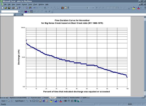
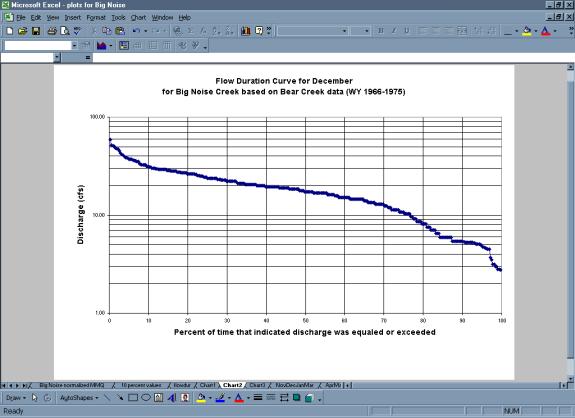
In Big Noise Creek, juvenile fish migrate upstream after the first fall freshets from November to January.  They migrate downstream in the late spring, April to June.  Also, winter adult Steelhead spawn from December to March (Jeff McEnroe, 6/3/02).  Hence, these are the months for which hydrologic estimates are needed.  Analysis results are shown in the following table.  Based on the results, the largest 10% exceedence probability flow occurs in January and is equal to 42 cfs. The culvert and any retrofitting structures should be designed to pass a flow of 42 cfs with a velocity of 2 ft/s if the passage criteria for juvenile fish are to be met at high flows.

Furthermore, the low flows during the same period must be considered to assure sufficient depth of water in the culvert for fish movement at winter baseflow conditions.  If fish are present between November and June, a flow of 2.7 cfs would be suitable to use in analysis of minimum flows for fish movement.  To achieve adequate depths at these small flows in an existing culvert, primarily designed to pass flood-peak flows, some form of retrofitting of the culvert bottom may be required.

Step 7:  Building confidence in flow estimates.  How good are the data and analyses?

One concern regarding the results of the hydrologic analysis for Big Noise Creek is the length of the period of record for Bear Creek.  The Bear Creek gage has only 10 years of streamflow data.  It may be useful to compare the Bear Creek data to a data set for a longer period of record to determine if the results generated using data from Bear Creek are representative of long-term patterns for the region.

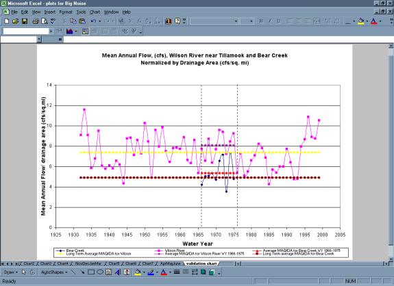
Wilson River has the longest period of record for the North Coast Basin.  By normalizing the mean annual discharge values for Bear Creek and Wilson River (to compress the data to a more easily visualized comparative size) and plotting Discharge/Unit Area vs. Water Year, the user can determine if the Bear Creek and Wilson River data follow a similar pattern. 

The following plot shows that the Bear Creek data does not occur in a particularly dry cycle or wet cycle and they follow the same general pattern as Wilson River.  Wilson River has a larger average value for MAQ/DA than Bear Creek.  This larger value could be due to the orographic effect discussed earlier, as the Wilson also has its headwaters in the Coast Range and flows west to the Pacific Ocean.  One could scale the Bear Creek values to the Wilson River values by using the ratio of the MAQ/DA values of each stream.  

(MAQ for Wilson River)*[(MAQ/DA for Bear Creek)/MAQ/DA for Wilson)] =

MAQ for Bear Creek.

Another comparison that can be made is to determine the average MAQ/DA for the Wilson River data for the concurrent water years (WY 1966-1975).  A ratio of the long-term average MAQ/DA to the short-term average MAQ/DA can be used to obtain the long-term average MAQ/DA for Bear Creek.

However, since the data for Bear Creek do not occur in an extreme cycle and the precipitation pattern in the Wilson River watershed may be slightly different than in the Bear Creek watershed, it may be more appropriate to use the flows estimated using only the Bear Creek data.

Step 8:  Summary of Results

• Flood Frequency Analysis
  • Used to design culvert capacity.

• Flow Duration Analysis
  • Used to determine design flow for fish passage concerns.