Analysis Techniques: Flood Analysis Tutorial with Instaneous Peak Flow Data (Log-Pearson Type III Distribution)

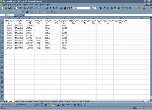
Download Data

View and print this webpage as a pdf file.

Step 1: Obtain streamflow data

• Obtain instantaneous peak streamflow data from the USGS web site.
  • Go to http://oregon.usgs.gov
  • Select Historical Water Data
  • Select Surface Water
  • Select Peaks
  • Check box under Site Identifier for Site Name and Submit
  • Type in Alsea under Site Name and select match any part and Submit
  • Select gage at TIDEWATER (140306500)
  • Select Tab-separated data
  • For the tutorial, copy the data for water years 1990 through 2000 into an Excel worksheet
  • Paste special as text (this will separate the data into columns)

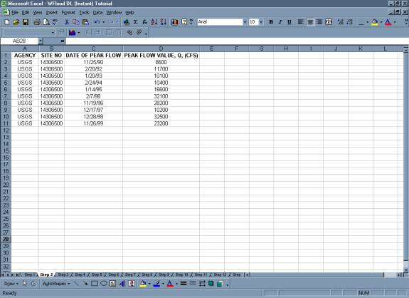
Step 2:  Organize the information in a table.

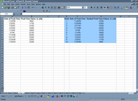
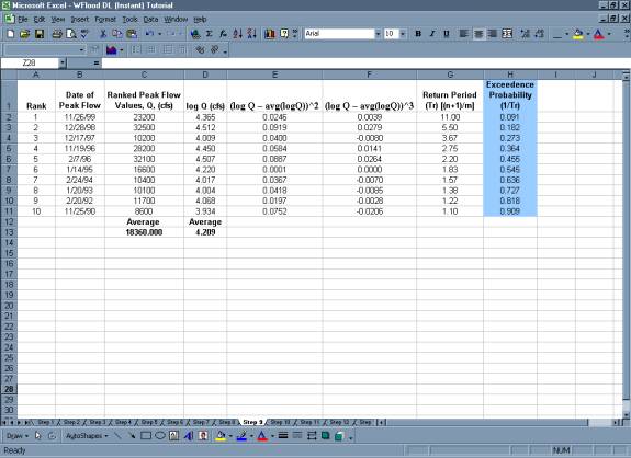
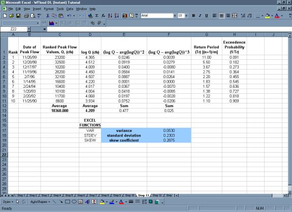
Step 3:  Rank the data from largest discharge to smallest discharge using the "sort" command.  Add a column for Rank and number each streamflow value from 1 to n (the total number of values in your dataset).

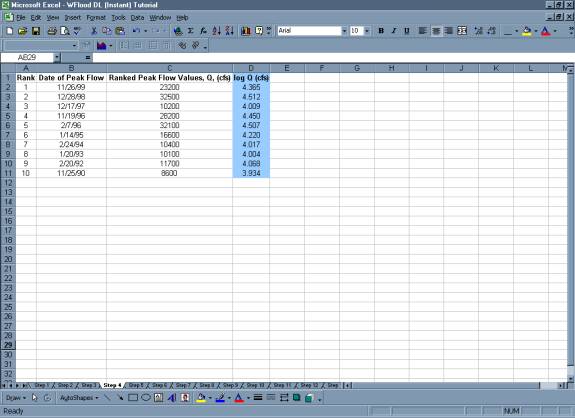
Step 4:  Create a column with the log of each max or peak streamflow using the Excel formula {log (Q)} and copy command.

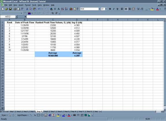
Step 5:  Calculate the Average Max Q or Peak Q and the Average of the log (Q)

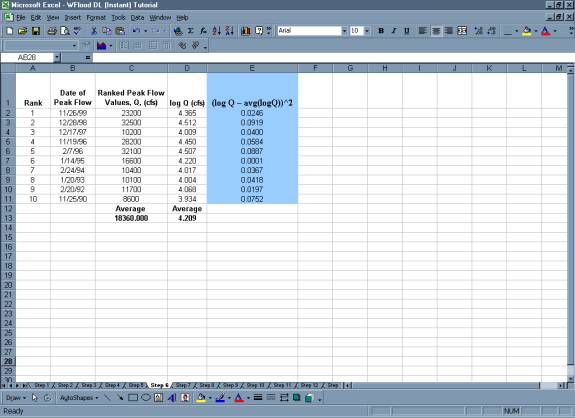
Step 6:  Create a column with the excel formula {(log Q – avg(logQ))^2}

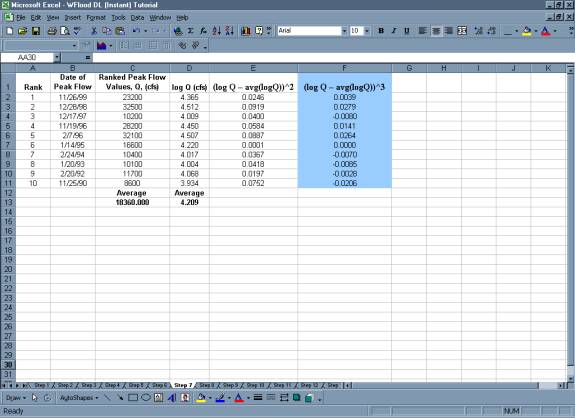
Step 7:  Create a column with the excel formula {(log Q – avg(logQ))^3

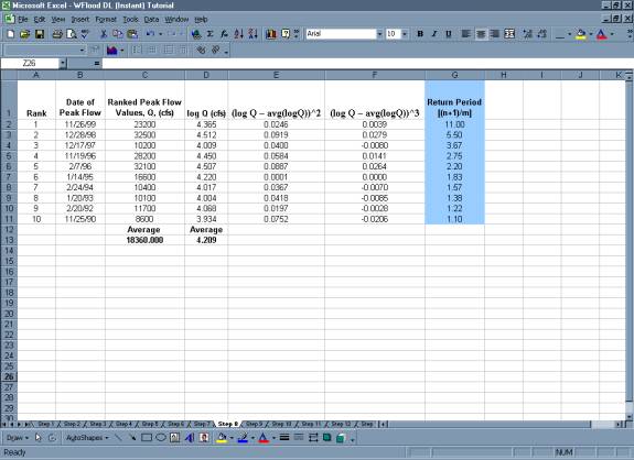
Step 8:  Create a column with the return period (Tr) for each discharge using the Excel formula {(n+1)/m}. 

Where n = the number of values in the dataset and m = the rank.

Step 9:  Complete the table with a final column showing the exceedence probability of each discharge using the excel formula {=1/Return Period or 1/Tr} and the copy command.

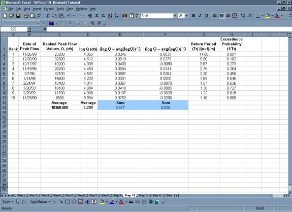
Step 10:  Calculate the Sum for the {(logQ – avg(logQ))^2} and the {(logQ – avg(logQ))^3} columns.

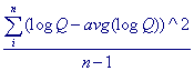
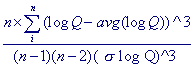
Step 11:  Calculate the variance , standard deviation , and skew coefficient as follows:

variance =  

standard deviation =   

skew coefficient =    

Excel functions can also be used to calculate the variance (=VAR( ) ), standard deviation (=STDEV( ) ), and skewness coefficient (=SKEW( ) ). Note that you use these formulas with the data in the log(Q) column.

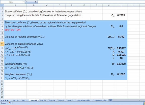
Step 12: Calculate weighted skewness

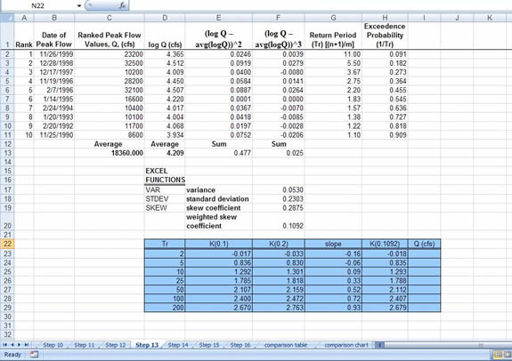
Show Me

Step 13:  Calculate K values

• Use the frequency factor table and the skew coefficient to find the K values for the 2,5,10,25,50,100, and 200 recurrence intervals. 
• If the skew coefficient is between two given skew coefficients in the table than you can linearly extrapolate between the two numbers to get the appropriate K value. To view the frequency factor table click on the "show me" link below.

Show Me

Step 14:  Using the general equation, list the discharges associated with each recurrence interval

general equation =

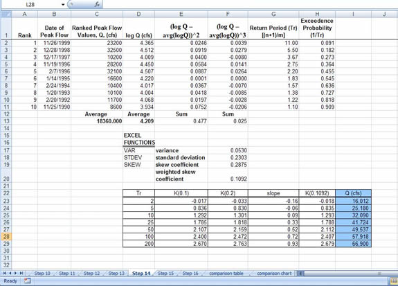
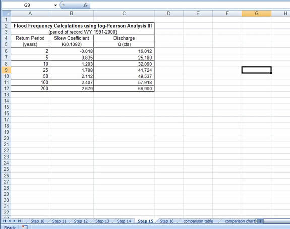
Step 15:  Create table of Discharge values found using the log – Pearson analysis

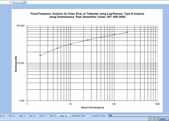
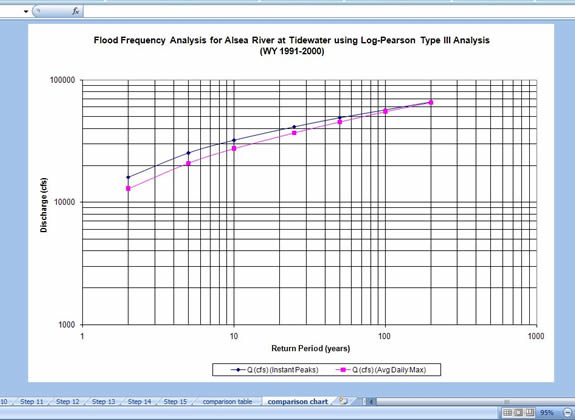
Step 16:  Create Plot

• Below is a comparison of flood frequency analysis completed using mean daily data versus instantaneous discharge data. As can be seen, had you completed this analysis using mean daily data, the result would have been an underestimation of the discharges, especially those associated with shorter return periods.