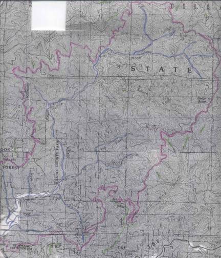
Examples: Wetland Habitat Assessment at the Kilchis River

Location:  The Kilchis River is located in the Northern Coast of Oregon.  The River flows southwest to Tillamook Bay, with headwaters in Tillamook State Forest (Lat 45.591^oN, Lon 123.644^oW) at an altitude of approximately 1000 feet above sea level.  The river flows through the northern portion of the city of Tillamook before entering the Bay.

Description of Project:  Heightened levels of erosion and flooding have been persistent problems in the city of Tillamook.  It has been shown that riparian wetlands act as sinks for material originating directly from upland areas and material in transport at high flow.  Wetlands are also known sites of exceedingly diverse, hydrology-dependent ecosystems that often accommodate managed and endangered species (Mitsch and Gosselink, 2000).  For these reasons, the health of a particular wetland in the Tillamook National Forest is to be assessed under a wetland evaluation and restoration initiative. The plan includes expanding the area of the wetland to serve a larger portion of the Kilchis River.  The Kilchis River does not have a streamflow gage.  

Objectives:  To determine the natural flood regime of the current wetland and choose native vegetation for the expansion accordingly. 

Plan of Action:  Conduct a comparison of nearby gaged systems to choose a data set to perform the hydrologic analyses for this project.  Develop a graph of the monthly discharge for an average year to know when inundation of the floodplain can be expected. Establish how often the river overtops its banks through a flood frequency analysis and flow duration curve.    Use data for a typical year to produce plots of mean daily discharge versus day of the year to find the times of the year when inundation is expected to occur. Determine on average, how many consecutive days this inundation occurs.  Choose plant species that thrive in the determined conditions. 

As you read through this example, you may wish to follow along with the analysis steps in an MS Excel file. You can download the data file by clicking here.

Step 1: Delineate the watershed and determine the drainage area of the Kilchis River using topographic maps.

Topographic maps used in this example are published by the U.S. Geological Survey (USGS) and were obtained for use here from the online map source topozone.com. The watershed was delineated using labeled ridges where possible.  For the areas of the watershed where the ridge tops are not clearly identified, headwaters of adjacent watersheds were used to determine the correct location of the drainage divide.  For this example, drainage area was calculated using an overlay grid of boxes with equivalent and known areas.  The boxes were counted and the number of boxes within the watershed multiplied by the area of an individual box.  The watershed drainage area was found to be 76 mi². 

Step 2:  Review the preliminary estimations page to determine a rough estimate of streamflow and precipitation values in this region.

The preliminary estimations for the North Coast will appear as follows:

Note that the values for monthly flow as a percentage of annual flow do not add up to 100%.  This is due to overlapping of drainage areas (i.e., nesting) of some or all gages used to calculate the percentages. 

The preliminary estimations for this basin show that the annual rainfall is approximately 80 inches.  The lower value of the range was chosen because the study site is at an elevation near sea level that would not be influenced by the orographic lift effect experienced higher in the mountain range.  Had the study site been located at or near the headwaters of the stream, the upper value would have been chosen.  With a drainage area of 76 mi² and use of the North Coast Basin annual discharge per unit area (4.98 cfs/mi²), the annual discharge is expected to be approximately 379 cfs.  The flow regime for a typical water year is anticipated to follow the general trend for areas west of the Cascade Mountains, namely, low flow during the summer months and peak flows during the winter months.  Furthermore, the most days of wetland inundation can be expected to occur during the months of December, January and February. 

Step 3:  Identify and list the characteristics of all nearby gages

A review of the table of USGS gages for the north coast of Oregon shows two gages that may be appropriate choices for providing the data with which to perform hydrologic analysis of the Kilchis River: Wilson and Trask Rivers.

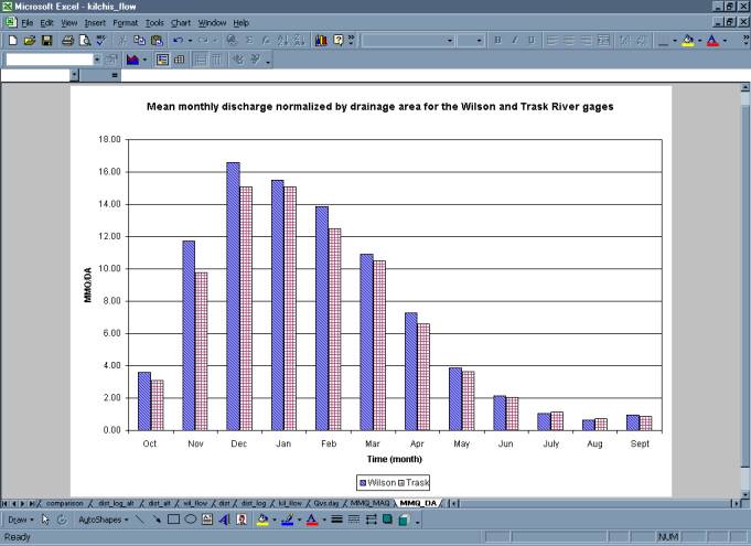
It is advantageous to select a gaged river that contains many years in the period of record.  The table shows the Wilson River gage as having 46 more years of data than the Trask gage, which suggests the use of data from the Wilson gage.  Normally, you would want to pick a gaged river with a drainage area similar to the drainage area of the study watershed; however, this is not always possible.  As can be seen, the drainage areas of both gaged rivers are much higher than that of the Kilchis.  Scaling will be needed in order to use either gage, but first further analyses must be conducted to determine which gage will be used.

Step 4:  Perform simple statistics on data to choose the most appropriate gage.

Mean monthly discharge for a typical water year, normalized by drainage area, is used in the selection process by showing the general pattern of streamflow for both gages.  As can be seen in the following figure, the pattern for the Wilson and Trask rivers are similar.  This means both gages exhibit the same flow regime that can be assumed to be typical of the region.  Although the Wilson River shows larger discharges throughout the rainy season, this is to be expected given its larger drainage area.  The important item to note here is the similarity in seasonal patterns. 

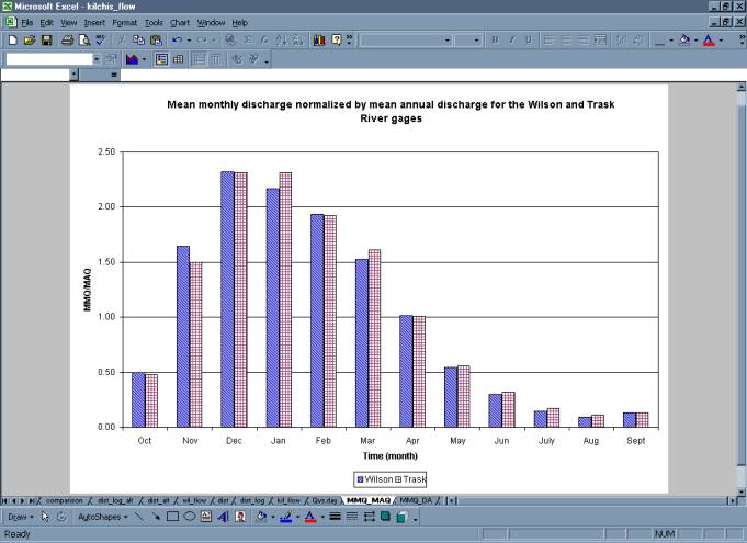
Plotting mean monthly discharge normalized by mean annual discharge for a typical water year shows that, in general, the discharge in both rivers are equivalent throughout most months.  The graph does suggest slight dissimilarities between the two sets of data, such that the Wilson may tend to rise toward the seasonal peak annual discharge earlier than the Trask.  The discrepancy could also have developed due to gaps (missing years) in period of record for one or both gages.  Because scaling will have to be done regardless, the flow regimes of the two rivers are comparable, and the Wilson has over twice the number of years in the period of record.  Therefore, the Wilson will most likely be used for the remainder of the analyses. However, both sets of data will be used for the flood frequency analysis to give one final comparison.

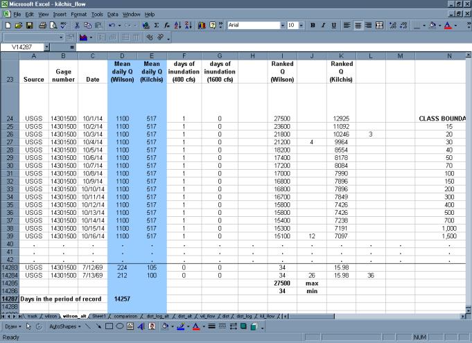
Step 5: Scale the Wilson River gage data to represent flows expected to be experienced by the smaller watershed of the Kilchis River.

The Kilchis River has a drainage area is considerably smaller than that of the Wilson River.  Using the following proportion, the values from the Wilson River gage were scaled down to better represent flows expected in the smaller Kilchis River:

(1)

Where A_K is the drainage area of the Kilchis River watershed, A_W the drainage area of the Wilson River watershed, Q_K the discharge scaled for the Kilchis River, and Q_W the discharge for the Wilson River as obtained from the USGS gage.  Solving this proportion for Q_K for each discharge value in the period of record results in the scaled Kilchis River data. The highlighted columns of the Microsoft Excel worksheet shows the results of the above calculation performed for each data point in the period of record.

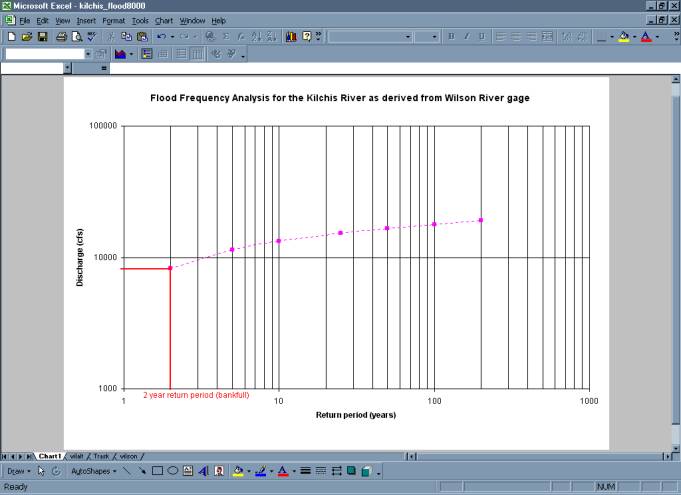
Step 6:  Conduct a flood frequency analysis to estimate at what magnitude of discharge inundation of the wetland will occur.

In order to estimate the magnitudes of large floods in the watershed, a Log Pearson type III flood frequency analysis regionalized for the northern coast of Oregon was conducted using the methods outlined in the Analysis Techniques section of this web site.  Instantaneous discharge values were used to conduct this analysis, as instantaneous values can briefly flood areas of concern.  After a survey of the study site has been conducted, the extent of inundation of the riparian wetland area due to floods of various return periods can be determined, as shown in the following figure.

Bankfull discharge is widely assumed to be associated with a flood with a 2-year return period, according to the plot that follows, bankfull discharge for the Kilchis River is approximately 8,000 cfs.  Bankfull discharge is the flow at which the channel is full to capacity (to the top of the banks).  Because it is more important for this project to know about the discharges associated with overtopping of the banks and inundation of the floodplain, a flow that may represent the threshold of general overbank flow is preferred.  Hence, any flow greater than 8,000 cfs will be considered a critical flow to investigate.  To get a more accurate figure for inundation, a survey of the channel adjacent to the wetland under study would need to be conducted.  A design flood can then be chosen according to the desired extent of inundation. 

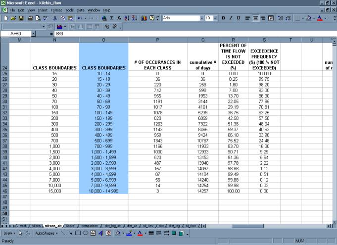
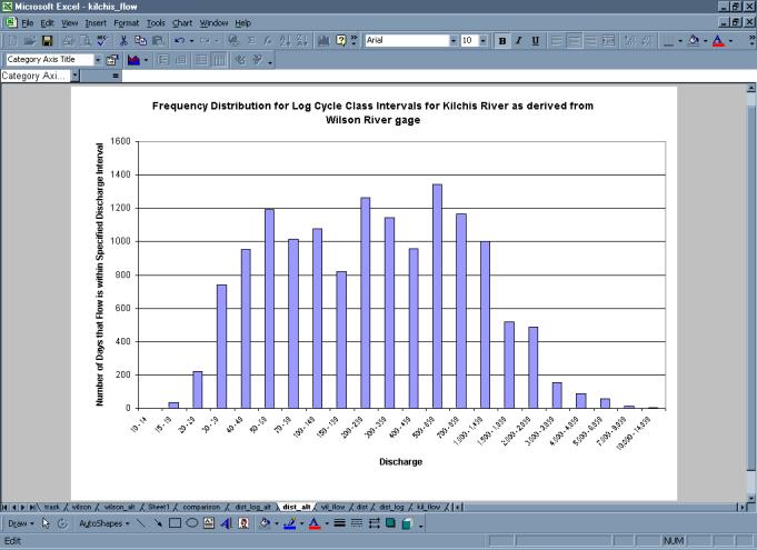
Step 7:  Sort scaled daily data in preparation of constructing a flow duration curve.

Before constructing the flow duration curve, a frequency distribution (histogram) was constructed for the sorted data to show the general spread of the data.  For this example, the data for the Kilchis has been sorted using the log cycles shown in the following Microsoft Excel spreadsheet. If improper intervals are chosen, the amount of information the flow duration curve can provide is diminished.  The elongated plateau of peak values suggest that the flow duration curve should be rather flat in the middle range.  This allows you to validate your methodology.

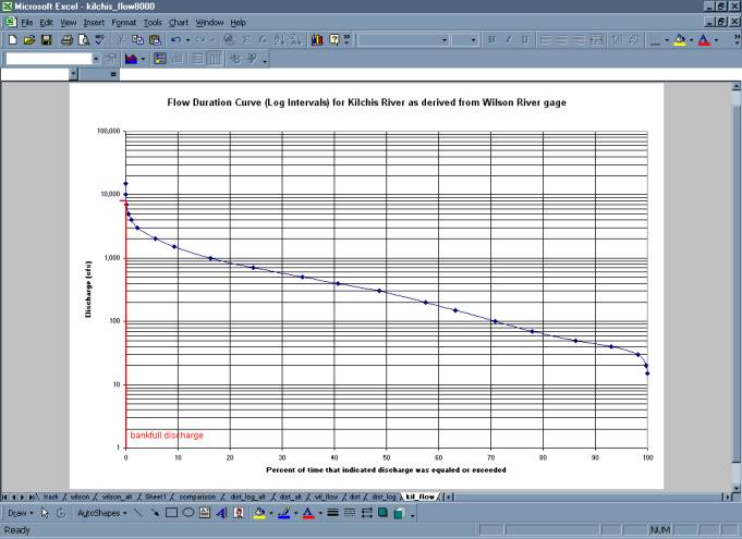
Step 8:  Construct a flow duration curve to predict what percent of time the wetland will be inundated.

As shown on the flood frequency curve, bankfull discharge is equaled or exceeded less than one percent of the time.  It would appear that if a seasonally flooded wetland were desired, mechanical means of flooding the wetland area would have to be employed.  A closer inspection of the daily values may expose additional information about how often pumping may be needed to artificially inundate the wetland.

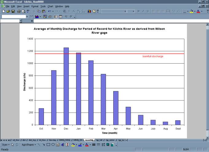
Step 9:  Develop a visual representation of the discharge associated with a typical water year

Using scaled monthly discharge values averaged over the entire period of record a plot of discharge vs. month for a typical water year was compiled.   From the following figure, it is concluded that if inundation does occur during a typical year, it will most likely occur during the months of December and January.  However, further analysis will improve the accuracy of this prediction. 

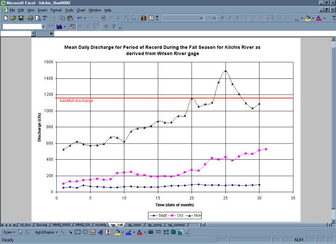
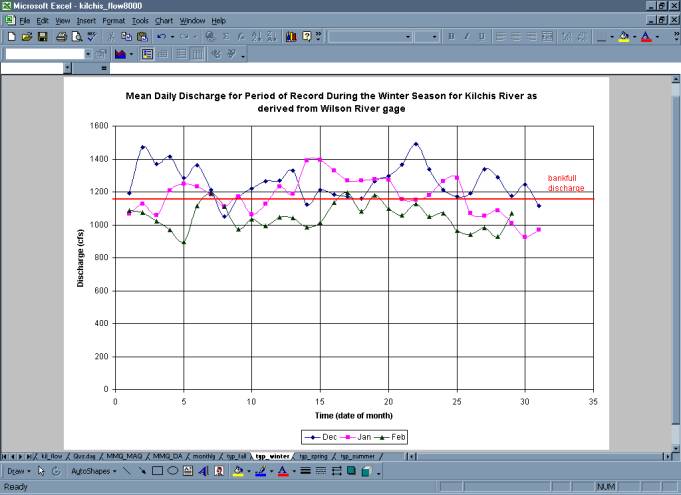
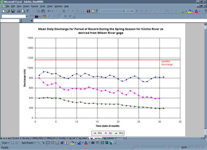
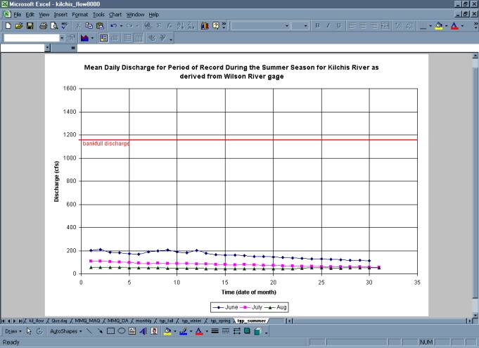
Step 10:  Conduct a monthly analysis to isolate the critical months for inundation and determine the average number of consecutive days inundation will occur.

Mean daily values by month validate the prior assumption that the flood regime of this area will create inundated vegetation mostly during the months of December and January.  However, the graph also shows a likely chance of overtopping periodically during February and late November.  With this new information, we can now predict that artificial flooding of the wetland during at least part of the rainy season may be unnecessary. Further analysis must be conducted to determine how often and for how many days to expect natural inundation versus how many days pumping will be implemented. 

Step 11:  Construct a table of discharges and dates for the flows that have a magnitude greater than 8000 cfs.

From the following table, it appears that the previous assumption that inundation may occur for a number of consecutive days was not correct.  We can conclude from the table that pumping must be used to flood the wetland area unless recharge due to groundwater poses a major influence on the hydrology of the site.

Days of Natural Inundation of Wetland:

Step 12:  Select vegetation that can withstand the predicted hydrologic regime.

There is a variety of native wetland vegetation in this region.  Two examples are camas lily and narrow-leaf mule’s-ears, which have both recently been successfully established in a Nature Conservancy restoration project (Nature Conservancy 2002).